TJCTF 2026 nesting write-up

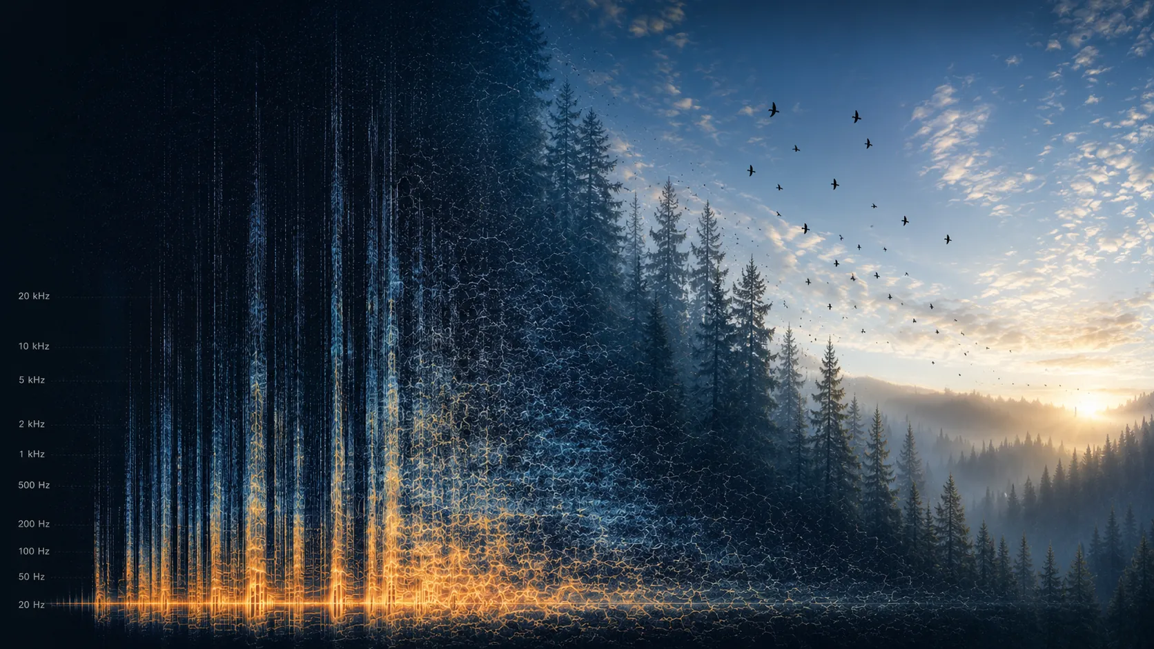
Hosted by the students of the Computer Security Club at Thomas Jefferson High School for Science and Technology in Northern Virginia, USA, this CTF challenge had a solve rate of about 5%. Let's find out what was nested inside. Along the way, we will explore media containers, digital signal processing, and the use of Python to generate spectrograms.

🏆 Update: This article was selected by the TJCTF 2026 organisers as one of the 5 winning write-ups of the competition! Huge thanks to the organisers for the recognition and the award!

Category: Forensics
Points: 470
Solves: 49 out of 954 teams
Author: Pinebery
Description: Who doesn’t like some forensics? Especially one about nests! :)
Attachments: nesting.mp4

Initial recon

We are given a 79 MB video file named nesting.mp4 showing a bird building a nest. Let’s start with some basic reconnaissance.

ffprobe nesting.mp4
[...]
Input #0, matroska,webm, from 'nesting.mp4':
  Metadata:
    ENCODER         : Lavf60.16.100
  Duration: 00:00:23.06, start: 0.000000, bitrate: 28850 kb/s
  Chapters:
    Chapter #0:0: start 0.624000, end 0.624000
[...]
    Chapter #0:11: start 22.505000, end 22.505000
  Stream #0:0: Video: h264 (High), yuv420p(tv, bt709, progressive), 1280x720 [SAR 1:1 DAR 16:9], 25 fps, 25 tbr, 1k tbn, start 0.021000 (default)
    Metadata:
      DURATION        : 00:00:23.021000000
  Stream #0:1: Audio: aac (LC), 48000 Hz, stereo, fltp (default)
    Metadata:
      DURATION        : 00:00:23.060000000
  Stream #0:2: Audio: pcm_f32le, 16000 Hz, 1 channels, flt, 512 kb/s (default)
    Metadata:
      DURATION        : 00:00:23.000000000
[...] 
  Stream #0:51: Audio: pcm_f32le, 16000 Hz, 1 channels, flt, 512 kb/s (default)
    Metadata:
      DURATION        : 00:00:23.000000000
  Stream #0:52: Subtitle: ass (ssa)
    Metadata:
      DURATION        : 00:00:23.000000000

Now we know that the video file is actually a Matroska container carrying the main video and audio streams, an additional 50 audio streams, 12 chapter pointers, and subtitles.

Except for the extra audio streams and chapters starting and ending on the exact same timestamps, it’s pretty standard content.

The obvious way of hiding a text flag would be to put it inside the subtitles, so that’s the first candidate for further examination.

Examining subtitles and chapters

First, let's just enable subtitles in a video player and see what they look like.

Whoa, these subtitles would require some serious speed-reading skills. At the same time, they look like random gibberish.

However, there are also chapter marks on the timeline. Maybe if we check what text is displayed at exactly those times, these short snippets could form a flag.

We need to extract the subtitles (stream #0:52) and chapter times first:

ffmpeg -i nesting.mp4 -map 0:52 subtitles.ass

The output file contains text and timestamps:

[Script Info]
Title: 
ScriptType: v4.00+
PlayResX: 1280
PlayResY: 720

[V4+ Styles]
Format: Name, Fontname, Fontsize, PrimaryColour, OutlineColour, BackColour, Bold, Italic, Alignment
Style: Default,Arial,60,&H00FFFFFF,&H00000000,&H64000000,0,0,5

[Events]
Format: Layer, Start, End, Style, Name, MarginL, MarginR, MarginV, Effect, Text
Dialogue: 0,0:00:00.00,0:00:00.05,Default,,0,0,0,,K,
Dialogue: 0,0:00:00.05,0:00:00.10,Default,,0,0,0,,ENF
Dialogue: 0,0:00:00.10,0:00:00.15,Default,,0,0,0,,ED
...
Dialogue: 0,0:00:22.85,0:00:22.90,Default,,0,0,0,,U
Dialogue: 0,0:00:22.90,0:00:22.95,Default,,0,0,0,,ICO
Dialogue: 0,0:00:22.95,0:00:23.00,Default,,0,0,0,,?

Next, the chapters. Let's use ffprobe for that and format the output as json. You may also use different ones like xml, csv, flat, ini or just default.

ffprobe -v quiet -show_chapters -print_format json nesting.mp4 > chapters.json

Content of the file:

{
    "chapters": [
        {
            "id": 7069736055514310406,
            "time_base": "1/1000000000",
            "start": 624000000,
            "start_time": "0.624000",
            "end": 624000000,
            "end_time": "0.624000"
        },
        ...
        {
            "id": -6304806635001805605,
            "time_base": "1/1000000000",
            "start": 22505000000,
            "start_time": "22.505000",
            "end": 22505000000,
            "end_time": "22.505000"
        }
    ]
}

Having both files, now we need to find out what text is displayed on each chapter's start.

import json

# Convert subtitle time format H:MM:SS.cs to seconds.
def parse_time(t_str):
    h, m, s = t_str.split(':')
    return int(h) * 3600 + int(m) * 60 + float(s)

# Load chapter start times
with open('chapters.json', 'r') as f:
    chapter_starts = [float(c['start_time']) for c in json.load(f)['chapters']]

# Parse subtitle start times, end times, and text
subs = []
with open('subtitles.ass', 'r') as f:
    for line in f:
        if 'Dialogue:' in line:
            parts = line[line.find('Dialogue:'):].strip().split(',', 9)
            if len(parts) == 10:
                subs.append((parse_time(parts[1]), parse_time(parts[2]), parts[9]))

# Match each chapter time to the corresponding subtitle text
flag = "".join(
    next((text for st, et, text in subs if st <= ct <= et), "") 
    for ct in chapter_starts
)

print(flag)

And the result is:

IAMNOTTHEFLAG.NOTYET!

We have a message saying it's not the flag, but it may become one. We got our first clue.

Extracting audio streams

The other odd thing about the video was that it had extra 50 audio streams. Let's extract and examine them. We use a bit of bash, because as powerful as FFmpeg is, it doesn't have a wildcard output flag (like output_%d.wav) yet.

for i in {2..51}; do
    printf -v padded_i "%02d" $i
    ffmpeg -v error -i nesting.mp4 -map 0:$i -c copy stream_${padded_i}.wav
    echo "Stream #0:$i saved as stream_${padded_i}.wav"
done

Now we have 50 .wav files saved, starting from stream_02.wav and ending on stream_51.wav.

When listening to them, we can hear really quiet sounds like birds chirping. Some waveforms also feature what sounds like a malformed voice reading something. For some reason it reminded me of "Aquarius" by Boards Of Canada.

One common technique is to hide messages in a waveform's spectrogram. The fastest way is to play the file with foobar2000 or load it into Audacity and switch the display mode to spectrogram or multi-view.

We can also use Librosa Python library to generate spectrograms.

import os
import glob
import matplotlib.pyplot as plt
import numpy as np
import librosa

os.makedirs("spectrograms", exist_ok=True)
my_dpi = 100

for wav_file in glob.glob("stream_*.wav"):
    y, sr = librosa.load(wav_file, sr=None)

    # Generate high-res Mel spectrogram and convert to decibels (log scale)
    S = librosa.feature.melspectrogram(y=y, sr=sr, n_fft=2048, hop_length=128, n_mels=512)
    S_dB = librosa.power_to_db(S, ref=np.max)
    
    # Extract exact dimensions (h, w) to map 1 data point to 1 pixel
    h, w = S_dB.shape
    plt.figure(figsize=(w / my_dpi, h / my_dpi), dpi=my_dpi)
    
    # Render using imshow to disable interpolation (pixel-perfect)
    plt.imshow(S_dB, origin='lower', aspect='auto', cmap='magma', interpolation='nearest')
    plt.axis('off')
    plt.subplots_adjust(left=0, right=1, bottom=0, top=1)
    
    # Save
    out_file = f"spectrograms/{wav_file[:-4]}.webp"
    plt.savefig(out_file, dpi=my_dpi, format='webp')
    plt.close()
    
    print(f"Saved: {out_file} ({w}x{h}px)")

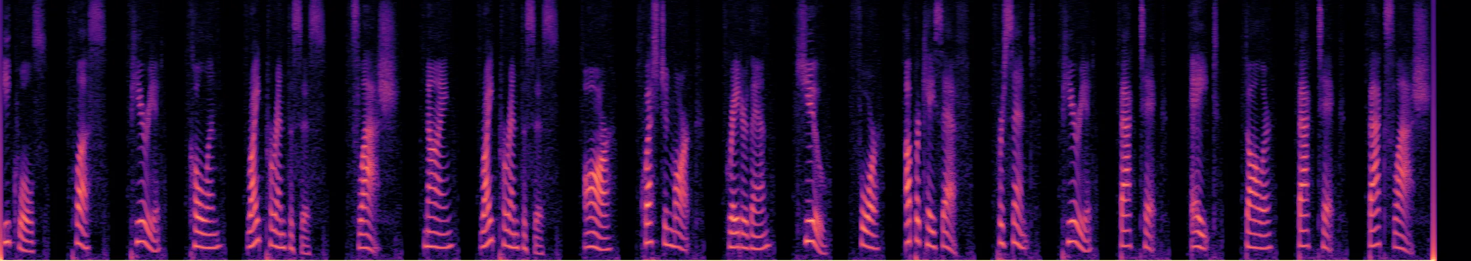
Some of the results:

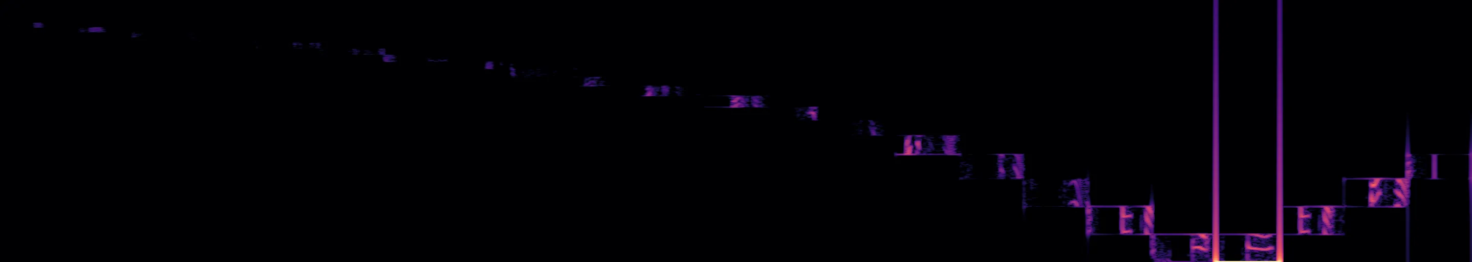
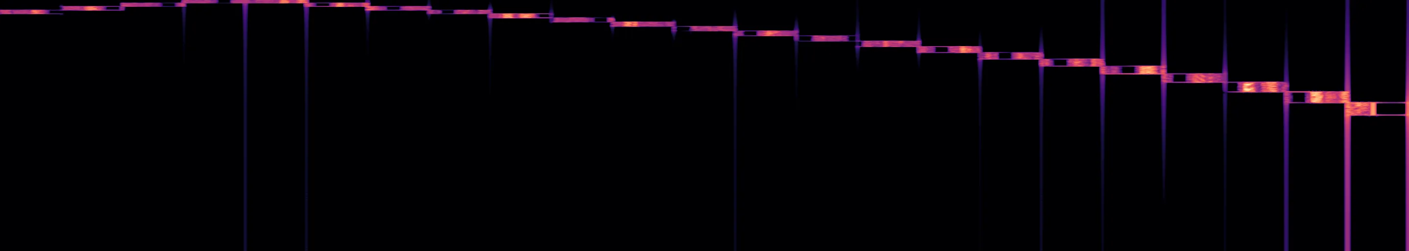
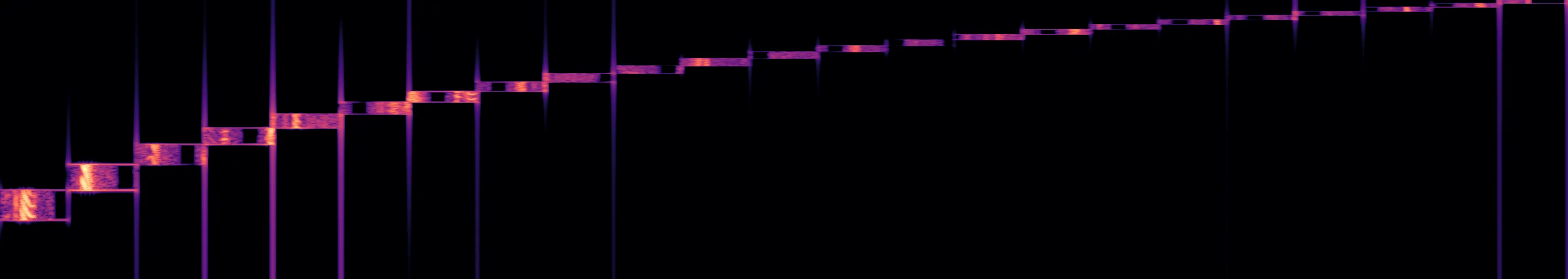
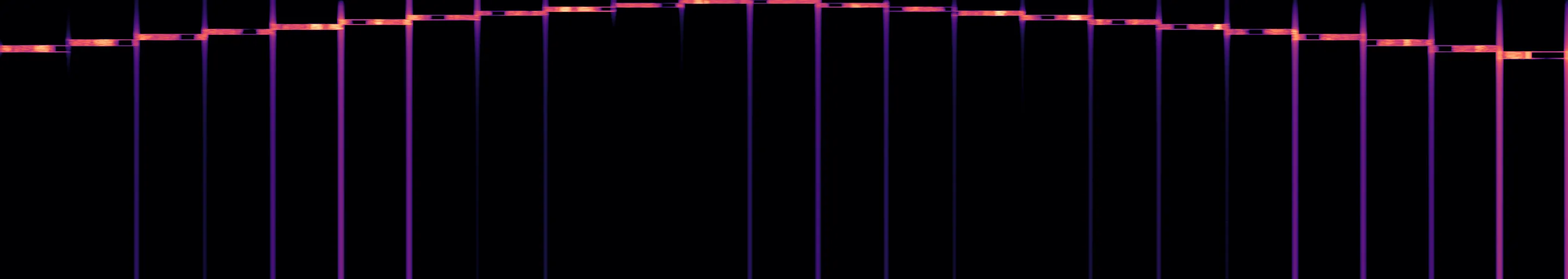
Looks like we get small fragments of a larger spectrogram. Maybe if we could add them together, a complete picture would appear. One solution would be to combine the images and then go back to the audio domain. The second one is to add the waveforms of all extra audio streams together, and then generate a completely new spectrogram.

The second option is easier, so let's sum all the waveforms. We should get something louder this time.

import numpy as np
from scipy.io import wavfile
import glob

# Grab all streams; assume they exist and are correctly named
files = sorted(glob.glob("stream_*.wav"))

# Initialize the mix with the first file
sr, mixed = wavfile.read(files[0])
mixed = mixed.astype(np.float32)

# Sum the remaining files, truncating to the shortest length to avoid indexing errors
for f in files[1:]:
    _, d = wavfile.read(f)
    min_len = min(len(mixed), len(d))
    mixed = mixed[:min_len] + d[:min_len]

# Normalize to [-1.0, 1.0] to prevent audio clipping
mixed /= np.max(np.abs(mixed))

wavfile.write("mixed_streams.wav", sr, mixed)
print("Saved mixed audio to mixed_streams.wav")

We got reconstructed recording of a woman reading out a sequence of symbols and characters:

Writing it down, we get:

=+.:)/9)r?>q4F%.`8$`\

This looks like it has the same lenght as the previous artifact that was not yet a flag:

IAMNOTTHEFLAG.NOTYET!

Since both strings have the same length, XOR is an obvious next step.

part_1 = "IAMNOTTHEFLAG.NOTYET!"
part_2 = r"=+.:)/9)r?>q4F%.`8$`\"".strip('"')
flag = "".join(chr(ord(a) ^ ord(b)) for a, b in zip(part_1, part_2))
print(flag)

Success, this time we get the real flag:

tjctf{ma7yr0shka4aa4}

We need to go deeper

Even though the challenge is already solved, there is still one more useful thing worth adding to the toolbox: a simple way to generate a classic waveform plot. Visualising the amplitude of a signal over time provides a different perspective from a spectrogram and is a fundamental technique in audio analysis.

import os
import glob
import matplotlib.pyplot as plt
import numpy as np
import librosa

os.makedirs("waveforms", exist_ok=True)

width_px = 1920
height_px = 600
my_dpi = 100 

for wav_file in glob.glob("stream_*.wav"):
    y, sr = librosa.load(wav_file, sr=None)
    
    # Convert pixels to inches for Matplotlib's figsize
    fig_width = width_px / my_dpi
    fig_height = height_px / my_dpi
    
    plt.figure(figsize=(fig_width, fig_height), dpi=my_dpi)
    
    # Generate the exact time coordinates for every single data point
    times = np.linspace(0, len(y) / sr, num=len(y))
    
    # Use standard plot with a thin line
    plt.plot(times, y, color="blue", linewidth=0.5)
    
    # Constrain the x-axis to exactly the start and end of the audio
    plt.xlim([0, times[-1]])
    
    plt.title(f"Waveform: {wav_file}")
    plt.xlabel("Time (seconds)")
    plt.ylabel("Amplitude")
    
    plt.tight_layout()
    
    # Construct output filename and save
    out_file = f"waveforms/{wav_file[:-4]}.webp"
    plt.savefig(out_file, dpi=my_dpi, format='webp')
    plt.close()
    
    print(f"Saved: {out_file} ({width_px}x{height_px}px)")

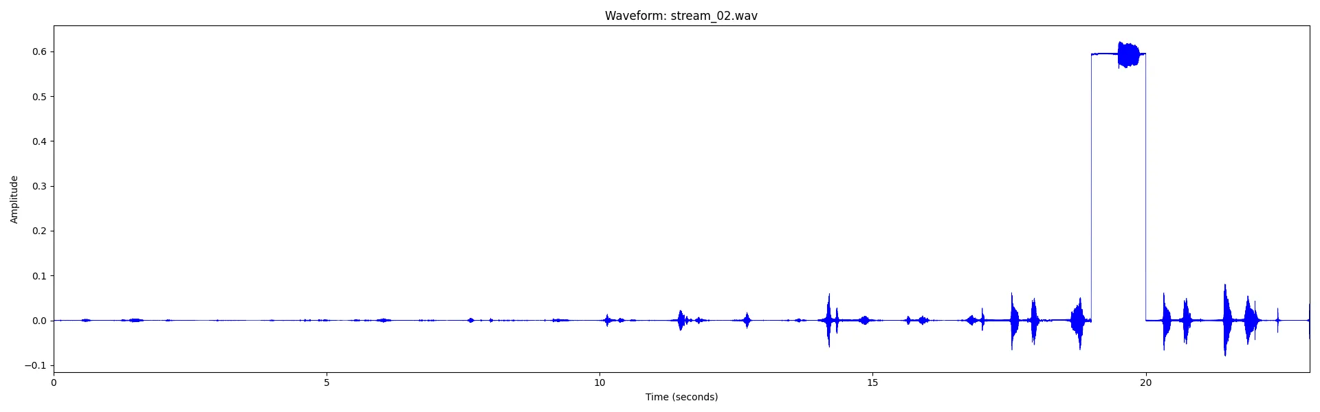
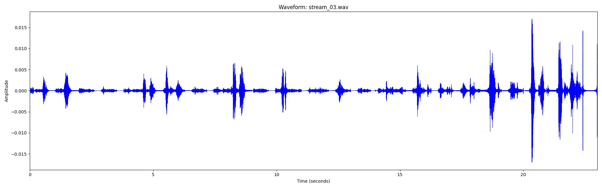
Did you notice the unusual amplitude shift in a section of the first waveform?

Summary

This challenge hid the flag across several different media layers inside a Matroska container. The subtitles and chapter markers provided the first clue, while the additional audio streams concealed the second part of the puzzle inside spectrogram fragments.

After reconstructing the hidden audio and extracting the encoded text, both artifacts could be combined with a simple XOR operation to recover the final flag.

The challenge was a nice example of how multimedia containers can carry much more than just visible video and audio data. It also demonstrated several useful forensic techniques, including stream enumeration with ffprobe, subtitle extraction, spectrogram analysis, and basic signal reconstruction with Python.

This write-up was originally published on mariuszbartosik.com and is reproduced here with permission from the author.